Variational Auto Encoders

To launch my technical blog’s math section, I’ll be presenting a concise overview of variational autoencoders (VAEs), with a particular emphasis on their mathematical connections to well-established algorithms. This is my first time writing a blog, and the key motivation is from the book “Cognitive Awakening: Bravely Breaking Out of Your Comfort Zone”, which will be shared seperately in a non-technical blog.

Echoing Plato’s Allegory of the Cave, a more principled understanding of the world may lie in the unobserved, high-dimensional variables that govern data generation. Even when a model of this underlying reality is conceptualized, the estimation of its parameters and latent variables remains a formidable challenge.

This blog explores three classes of probabilistic models. We begin with the straightforward Gaussian distribution, amenable to parameter estimation via Maximum Likelihood Estimation (MLE). We then progress to Gaussian Mixture Models, which necessitate iterative inference of latent component assignments and parameter estimation. Finally, we address complex models where latent variable estimation becomes intractable, encompassing recent advancements in neural network-based generative AI, such as U-Nets and Transformers.

1. Warmup: likelihood maximization with Gaussian distribution

Consider a set of observations \(\mathbf{X} = \{X_i\}_{i=1}^N\) sampled from Gaussian distribution \(X_i \sim \mathcal{N}(\mu, \sigma^2)\), the likelihood of the observation can be modeled as

\[L(\mu, \sigma^2) = \prod_{i=1}^{n} \frac{1}{\sqrt{2\pi\sigma^2}} \exp\left(-\frac{(X_i - \mu)^2}{2\sigma^2}\right).\]

The log-likelihood of the observation can be experssed as

\[\log L(\mu, \sigma^2) = -\frac{n}{2} \log(2\pi\sigma^2) - \frac{1}{2\sigma^2} \sum_{i=1}^{n} (X_i - \mu)^2\]

In this case, model parameter is defined as \(\theta = (\mu,\sigma^2)\). The optimal estiamte of mean and variance can be obtained taking partial derivate of the log-likelihood

\[\begin{aligned} \frac{\partial}{\partial \mu} \log L &= \frac{1}{\sigma^2} \sum_{i=1}^{n} (X_i - \mu)\\ \frac{\partial}{\partial \sigma^2} \log L &= -\frac{n}{2\sigma^2} + \frac{1}{2\sigma^4} \sum_{i=1}^{n} (X_i - \mu)^2 \end{aligned}\]

Note: here we can first solve the estimated mean \(\hat{\mu}\) and substitute it back to the second equation for the closed-form solution of \(\sigma^2\). However, since we don’t have the ground truth mean and estimate it instead, we may need to apply Bessel’s correction to the estimate of the variance.

2. Gaussian Mixture Model

Now we consider a Gaussian Mixture Model (GMM), where the probability of data distribution is expressed as

\[P(x, \theta) = \sum_{k=1}^{K} \pi_k \mathcal{N}(x | \mu_k, \Sigma_k)\]

where

• \(K\) is the number of Gaussian components.
• \(\pi_k\) is the mixture weights (prior probabilities of each component), satisfying \(\sum_{k=1}^{K} \pi_k = 1\)
• \( \mathcal{N}(x | \mu_k, \Sigma_k)\) is a multivariate Gaussian distribution with mean \(\mu_k\) and covariance matrix \(\Sigma_k\).

For this model, the goal is to estimate the parameter set \(\mathbf{\theta} = \{\pi_k, \mu_k, \sigma_k\}_{k=1}^K\) from the data set \(\mathbf{X}\). In the Gaussian Mixture Model, it’s challenging to obtain a closed-form optimal estimate of the model parameters. To make the estimation more tractable, we introduce a set latent vectors \(\mathbf{Z} = \{ Z_i \}_{i=1}^N\) for each data point, where \(z_{ik}\) is the binary indicator variable indicating whether belongs to component \(k\). And the complete-data log-likelihood is defined as

\[\sum_{i=1}^N \log P(x_i, Z_i, \theta) = \sum_{i=1}^N \sum_{k=1}^K z_{ik} \left[ \log \pi_k + \log \mathcal{N}(x_i|\mu_k, \Sigma_k) \right]\]

However, the marginal likelihood is defined as \(\mathcal{L}_c(\theta) = \sum_{i=1}^N \log P(x_i, \theta)\) and we need to posterior probability \(P(Z_i \vert x_i, \theta)\) to accomplish the conversion. Without the knowledge of model parameter \(\theta\), it’s very challenging to estimate the conditional distribution of latent variable $z$ only given a set of observations \(\mathbf{X} = \{X_i\}_{i=1}^N\). And the model parameter \(\theta\) can only be optimized correctly with latent variable estimation. Then, this issue becomes a chicken-egg problem.

And the goal of Expectation-Maximization (EM) algorithm is to optimize the \(\theta\) and \(\mathbf{Z}\) iteratively.

3. Expectation-Maximization (EM) Algorithm

Generally speaking, EM algorithm is operating in the following way

• E - Step: Given the previous model parameter \(\theta^t\) and the distribution of latent \(\mathbf{Z}\), we estimate the log likelihood for the set of data points \(\mathbf{X}\), using \(Q(\theta, \theta^t) = \mathbb{E}_{Z|X, \theta^t}[\mathcal{L}_c(\theta)].\)
• M - Step: Update the parameter by \(\theta^{t+1} = \arg\max Q(\theta, \theta^t)\)

3.1 Implementation of E step

In this specific case, the log likelihood in the E-step is expressed as

\[\begin{aligned} Q(\theta, \theta^t) & = \mathbb{E}_{Z|X, \theta^t} \left[ \sum_{i=1}^N \log P(x_i , Z_i, \theta) - \log P( Z_i |x_i, \theta^t) \right]\\ & = \mathbb{E}_{Z|X, \theta^t} \left[ \sum_{i=1}^N \sum_{k=1}^K z_{ik} \left( \log \pi_k + \log \mathcal{N}(x_i|\mu_k, \Sigma_k) \right) \right] - C\\ & = \sum_{i=1}^N \sum_{k=1}^K \gamma_{ik} \left( \log \pi_k + \log \mathcal{N}(x_i|\mu_k, \Sigma_k) \right) - C, \end{aligned}\]

where \(C\) is a constant value unaffected by \(\theta\), \(\gamma_{i,k}\) is the expected value of \(z_{i,k}\), or the probability the the data sample \(i\) belongs to cluster \(k\).

It’s impotant to note in the E-step, the conditional distribution \(P(Z_i \vert x_i, \theta^t)\) can be easily caculated with model parameter. Then it’s used to approximate the unconditional latent variable distribution \(P( Z_i \vert \theta^t)\).

Given our estimated model parameter \(\mathbf{\theta}^t = \{\pi_k, \mu_k, \sigma_k\}_{k=1}^K\), the expected values can be estimated in the following form

\[\gamma_{ik} = \frac{\pi_k \mathcal{N}(x_i|\mu_k, \Sigma_k)}{\sum_{j=1}^K \pi_j \mathcal{N}(x_i|\mu_j, \Sigma_j)}\]

3.2 Implementation of M step

Next we obtain the updated model parameters by setting the subgradient of the log-likelihood as zero, where

\[\frac{\partial Q}{\partial \pi_k} = 0, \frac{\partial Q}{\partial \mu_k} = 0, \frac{\partial Q}{\partial \Sigma_k} = 0, \forall k \in [N].\]

First, given the fact \(\sum_{k=1}^K \pi_k = 1\), we can estimate the mixture weights by introducing Lagrange multipliers

\[\frac{\partial}{\partial \pi_k} \left[ Q(\theta, \theta^t) + \lambda \left( 1 - \sum_{k=1}^K \pi_k \right) \right] = 0.\]

And its closed form solution is \(\pi_k = \frac{\sum_{i=1}^N \gamma_{ik}}{N}\). Next, the mean and variance of each components can be estimated by

\[\begin{aligned} \frac{\partial Q}{\partial \mu_k} &= \sum_{i=1}^N \gamma_{ik} \frac{\partial}{\partial \mu_k} \log \mathcal{N}(x_i|\mu_k, \Sigma_k) \Rightarrow \sum_{i=1}^N \gamma_{ik} \Sigma_k^{-1} (x_i - \mu_k) = 0\\ \frac{\partial Q}{\partial \Sigma_k} &= \sum_{i=1}^N \gamma_{ik} \frac{\partial}{\partial \Sigma_k} \log \mathcal{N}(x_i|\mu_k, \Sigma_k) \Rightarrow -\frac{1}{2} \sum_{i=1}^N \gamma_{ik}\left[ \Sigma_k^{-1} - \Sigma_k^{-1} (x_i - \mu_k)(x_i - \mu_k)^T \Sigma_k^{-1} \right] = 0 \end{aligned}\]

Then the closed-form solution of the mean and variance can be obtained as

\[\begin{aligned} \mu_k = \frac{\sum_{i=1}^N \gamma_{ik} x_i}{\sum_{i=1}^N \gamma_{ik}}, \;\; \Sigma_k = \frac{\sum_{i=1}^N \gamma_{ik} (x_i - \mu_k)(x_i - \mu_k)^T}{\sum_{i=1}^N \gamma_{ik}} \end{aligned}\]

4. Stochastic Gradient Variational Bayes

The derivation of EM algorithm heavily hinges on the extimation of posterior probability of latent variable \(Z\), conditioned on the model parameter \({\theta}\). This is expressed as

\[P(z_{i,k} = 1 |X, \theta^t) = \frac{\pi_k \mathcal{N}(x_i|\mu_k, \Sigma_k)}{\sum_{j=1}^K \pi_j \mathcal{N}(x_i|\mu_j, \Sigma_j)}\]

For a general class of parametric distributions \(P(Z, \theta)\) and \(P(X \vert Z, \theta)\), obtaining the posterior distribution \(P(Z \vert X, \theta)\) is typically computationally intractable. This is due to the Bayes’ formula requiring the marginal likelihood \(P(X, \theta)\). Thus, instead of deriving a closed-form posterior, such posterior is approximated by another parametric distribution \(q(X \vert Z, \phi)\) and the log-likelihood of the dataset can be rewritten as

\[\begin{aligned} \mathcal{L}_c(\theta) &= \sum_{i=1}^N \log P(x_i, \theta) = \mathbb{E}_{Z|X, \phi} \left[\sum_{i=1}^N \log P(x_i, \theta) \right]\\ &= \mathbb{E}_{Z|X, \phi} \left[ \sum_{i=1}^N \log P(x_i, Z, \theta) - \log P(Z \vert x_i, \phi) \right] + \mathbb{E}_{Z|X, \phi} \Bigl[ \log P(Z \vert x_i, \phi) - \log P(Z \vert x_i, \theta) \Bigr] \\ &= \mathcal{L}_{ELBO}(\theta,\phi) + D_{KL}\bigl( P(Z \vert X, \theta) \| (P(Z \vert X, \phi) \bigr) \end{aligned}\]

The first term in the right hand side is also known as evidence lower bound (ELBO). Due to the non-negativity of KL divergence, for any model parameter \(\theta\), the marginal likelikood is maximimized iff \(P(Z \vert X, \theta) == P(Z \vert X, \phi)\).

4.1 Stochastic Gradient Variational Bayes (SGVB)

For each data sample \( x_i\) ELBO objective can be written as

\[\mathcal{L}_{ELBO}(\theta,\phi, x_i) = \mathbb{E}_{Z|x_i, \phi} \left[ \log P(x_i, Z, \theta) - \log P(Z \vert x_i, \phi) \right]\]

By reparameterizing the latent variable as a mapping function plus a certain noise, the latent variable can be expressed as

\[z = g_{\phi}(x, \epsilon) \;\;\; \text{with} \;\;\; \epsilon \sim p(\epsilon)\]

Then we can get a stochastic version of ELBO by sampling from the noise distribution, which is

\[\begin{aligned} \mathcal{L}^A_{ELBO}(\theta,\phi, x_i) &= \frac{1}{L} \sum_{l=1}^L \left[ \log P(x_i, z_{i,l}, \theta) - \log P(z_{i,l} \vert x_i, \phi) \right] \\ s.t. \;\;\; z_{i,l} &= g_{\phi}(x_i, \epsilon_{i,l}) \;\;\; \text{with} \;\;\; \epsilon_{i,l} \sim p(\epsilon) \end{aligned}\]

Note:

Without the reparameterization technique, to obtain the gradient \(\nabla_{\phi} \mathbb{E}_{q_{\phi}(z)}[f(z)]\), the standrad SGVB estimator uses the following property

\[\nabla_{\phi} \Bigl( \log q_{\phi}(z) f(z)\Bigr) = \nabla_{\phi} \Bigl( \log q_{\phi}(z) \Bigr) f(z) = \frac{\nabla_{\phi} q_{\phi}(z)}{q_{\phi}(z)} f(z)\]

Thus, the gradient of expected value \( f(z) \) can be estimated without explicitly differentiating the function, which is

\[\nabla_{\phi} \mathbb{E}_{q_{\phi}(z)}[f(z)] = \mathbb{E}_{q_{\phi}(z)}[f(z) \nabla_{\phi} \log q_{\phi}(z)]\]

4.2 Auto Encoding Variational Bayes (AEVB)

In the SGVB method, for each data sample \(xi\), both of these two log likelihoods are affected by the randomness of latent variable \( z{i,l}\). To make the learning and inference more efficient, the ELBO can be rewritten as

\[\mathcal{L}_{ELBO}(\theta,\phi, x_i) = - D_{KL}(P(Z \vert x_i, \phi) \| P(Z, \theta)) + \mathbb{E}_{Z|x_i, \phi} \left[ \log P(x_i \vert Z, \theta) \right]\]

In my opinion, there are two key advantages in brought by AEVB method. First, the KL divergence can be calculated in closed-form for Gaussian distributions and the sampling variance only exists in the last term. Second, the distribution of latent variable is usually known as a prior (e.g. Gaussian for image generation), while the SGVB method doesn’t fully utilize this information. Similar to the SGVB method, a stochastic version of the AEVB formula can be approximated by

\[\begin{aligned} \mathcal{L}^B_{ELBO}(\theta,\phi, x_i) &= - D_{KL}(P(z \vert x_i, \phi) \| P(z, \theta)) + \frac{1}{L} \sum_{l=1}^L \left[ \log P(x_i \vert z_{i,l}, \theta) \right] \\ s.t. \;\;\; z_{i,l} &= g_{\phi}(x_i, \epsilon_{i,l}) \;\;\; \text{with} \;\;\; \epsilon_{i,l} \sim p(\epsilon), \end{aligned}\]

where the KL-divergence can be obtained by comparing the mean and variance estimate from the encoder network \(\phi\) with the prior latent distribution.

5. Recap

This blog explores the problem of finding a model that optimally approximates the distribution of data samples, \(\mathbf{X} = \{X_i\}_{i=1}^N\), specifically by maximizing the marginalized log-likelihood. To achieve this, we consider latent variable models, where unobserved variables are assumed to generate the data. We then discuss how Expectation-Maximization (EM) algorithms and Variational Bayes methods estimate these latent variables and model parameters under different settins.

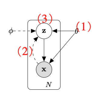
As illustrated in the figure, maximizing the marginalized probability requires statistical approximation of three key elements: 1) the model parameters, \(\theta\); 2) the posterior distribution, \(P(Z \vert X, \theta\); and 3) the distribution of the latent variable given model parameters, \(P(Z, \theta) \).

In Gaussian Mixture Models (GMMs), estimating the posterior distribution (2) is relatively straightforward given the model parameters (1) and the distribution (3), enabling iterative optimization of (1) and (3). Variational Bayes methods, however, face challenges in estimating (2), necessitating an additional approximation. Stochastic Gradient Variational Bayes (SGVB) methods address this by jointly optimizing (1), (2), and (3) using Monte Carlo estimates of the Evidence Lower Bound (ELBO). Auto-encoding Variational Inference (AEVB) further reduces variance by imposing a constraint on (3), a technique widely employed in modern generative models.