Balanced trees

# CS 10C - Balanced trees

![:newline]

.Huge[*Prof. Ty Feng*]

![:newline]

.Large[UC Riverside - WQ 2026]

![:newline 6]

![:scale 40%](../utils/style/ucr_cs_logo.png)

![:scale 45%](images/balance-bst-tweet.webp)

---

# Recap on BST

---

## Height of tree

![:flush 3]

### Proof (kind of)
Considering a perfect binary tree of height $h$
- Each level has exactly twice as many nodes as the previous level
- The first level has only one node (the *root* node)
- The total number of nodes is equal to the sum of the nodes on all levels
$$$N = 1 + 2 + 4 + 8 + ... + 2^h = 2^{h+1} - 1$$$
- The height is therefore
$$$h = \log_2(N + 1) - 1 = O(\lg N)$$$

???

- x = log2(n) <=> 2^x = n
- Solution
    * $2^{h+1} - 1 = N$
    * $2^{h+1} = N + 1$
    * $h+1 = \lg(N + 1)$
    * $h = \lg(N + 1) - 1$

---

## Complexity

![:flush 1]

## Conclusion
- If BST is guaranteed to stay balanced, the worst-case complexity is guaranteed
  to be $O(\lg N)$
- So, how do we make a BST stay balanced?

---

# Ideas

.lcol[
## Same population from root?
- Maintain same number of nodes on each side of root
- But...
![:scale 50%](images/binary_tree_same_pop.svg)
]

???

- So, what does it mean for a tree to stay balanced?

![:newline 1]
- Doesn't force tree to be balanced internally on either side
- Here, difference in heights

.rcol[
## Same height from root?
- Maintain same height on each side of root
- But...
![:scale 50%](images/binary_tree_same_height.svg)
]

???

- Same height, but still not balanced

.lcol[
## Same height for each node?
- For each node, maintain same height in left and right subtrees
- But...
![:scale 50%](images/binary_tree_perfect.svg)
]

???

- Only perfect trees can respect this condition!

.rcol[
## Requirements
Must find a good **balance condition**
- Easy to maintain
- Depth of BST stays $O(\lg N)$
- Not too rigid
]

???

- In this class, we will focus on four balanced trees
    * AVL and RB trees, which are both great options for in memory trees
    * B-trees, great option for on-disk trees
    * Splay trees in discussion next week

---

# AVL trees

---

## Definition

- Published in 1962, by **A**delson-**V**elskii and **L**andis
    - *First self-balancing BST data structure to be invented*
![:newline 1]
- AVL trees are height-balanced binary search trees
- For each node, the height of its left subtree and the height of its right
  subtree can differ by **at most** 1
    - Such difference value is called the node's *balance factor*

???

- Over 60 years ago

![:newline 1]

### Example

![:scale 65%](images/avl_example.svg)

---

## Non-AVL trees

For each node:
- Determine its height
- Determine its balance factor
- If balance factor is not -1, 0 or 1, then tree is not AVL

![:newline 2]

### Examples
.lcol[
![:scale 90%](images/non-avl_example1.svg)
]

???

- First tree
    - balance factor at node 18: +2
    - balance factor at node 43: +2
- Second tree
    - balance factor at node 43: -2

![:newline 2]
- Live quiz!

---

## Operations

.lcol[
- Query operations stay unchanged
    - `Contains()`, `Min()`, `Max()`
- But worst-case complexity is now $O(\lg N)$!
    - Because AVL trees are guaranteed to be height-balanced
]

![:flush 2]

.lcol[
- Operations that *could* alter the balance of the tree must be slightly
  modified
    - `Insert()`, `Remove()`
- Rebalancing after insertion or removal if balance condition is broken
]

---

## Simple rebalancing

.lcol.small[
- Regular BST (*recursive*) insertion into AVL tree
![:scale 90%](images/avl_simple_rebalancing_1.svg)
]

.rcol.small[
- **Retracing**: check every ancestor's balance factor
![:scale 90%](images/avl_simple_rebalancing_2.svg)
]

???

- As we will see later, there are different scenarios we need to deal with
- Here, we notice that both balance factors have same sign (+1 and +2), which
  tells us how to fix the problem

![:flush]

.lcol.small[
- Swap unbalanced parent with "heavy" child through rotation
![:scale 90%](images/avl_simple_rebalancing_3.svg)
]

.rcol.small[
- Tree is back to being AVL
![:scale 100%](images/avl_simple_rebalancing_4.svg)
]

---

## Single rotation right

- Imbalance caused by either
    - Height decrease in subtree W (removal)
    - Height increase in subtree T (insertion)
- Need a *right rotation* to rebalance left-heavy tree
    - $O(1)$ operation

---

## Single rotation left

- Imbalance caused by either
    - Height decrease in subtree T (removal)
    - Height increase in subtree W (insertion)
- Need a *left rotation* to rebalance right-heavy tree
    - $O(1)$ operation

---

---

# Recap

.rcol[
### Query ops
- Unchanged query operations
- Guaranteed $O(\lg(N))$
![:scale 80%](images/avl_ops_unchanged.svg)
]

![:flush 1]

### Simple rebalancing

.lcol[
- Solved by a single rotation
![:scale 80%](images/avl_simple_rebalancing_1.svg)
]
.rcol[
![:scale 90%](images/avl_simple_rebalancing_4.svg)
]

???

- Imbalance caused by insertion: +1 at node 54, +2 at node 93
- Last time, started studying concepts
- Today, finish concepts and start with C++ implementation

---

---

## Complex rebalancing

.lcol.small[
- Retracing shows imbalance; but child's balance factor has *opposite* sign
![:scale 85%](images/avl_complex_rebalancing_1.svg)
]

???

- Show on blackboard what would happen with right rotation (like we solved the
  imbalance from previous example)

.rcol.small[
- Need to first rotate child with heavy grandchild
![:scale 85%](images/avl_complex_rebalancing_2.svg)
]

![:flush]

.lcol.small[
- Only then rotate unbalanced parent with heavy child
![:scale 90%](images/avl_complex_rebalancing_3.svg)
]

.rcol.small[
- Tree is back to being AVL
![:scale 100%](images/avl_complex_rebalancing_4.svg)
]

---

.lcol[
## Double rotation: left-right
.small[
- Imbalance caused by either
    - Insertion of node Y
    - Height decrease in subtree W
    - Height increase in subtrees U or V
- Inner child Y of X is deeper than T
- Need a *left rotation* to rebalance inner right-heavy subtree
- Followed by a *right rotation* to rebalance left-heavy tree
]
]

---

.lcol[
## Double rotation: right-left
.small[
- Imbalance caused by either
    - Insertion of node Y
    - Height decrease in subtree T
    - Height increase in subtrees U or V
- Inner child Y of Z is deeper than W
- Need a *right rotation* to rebalance inner left-heavy subtree
- Followed by a *left rotation* to rebalance right-heavy tree
]
]

---

# AVL trees

---

## Implementation: data structure

- Based on BST, unchanged for all *query* methods
    - `Contains()`, `Min()`, `Max()`
- Node structure increased to contain the height information
- A few extra internal methods for self-balancing purposes

![:newline 1]

.lcol60.footnotesize[

```C
template <typename T>
class AVL {
...
  struct Node{
    T key;
    int height;
    std::unique_ptr<Node> left;
    std::unique_ptr<Node> right;
  };
  std::unique_ptr<Node> root;
...
  // Helper methods for the self-balancing
  int Height(Node *n);
  void RotateRight(std::unique_ptr<Node> &prt);
  void RotateLeft(std::unique_ptr<Node> &prt);
  void Retrace(std::unique_ptr<Node> &n);
};

```

![:filename](avl.h)

]

???

- `prt` stands for "parent"

.rcol40.small[

```C
template <typename T>
int AVL<T>::Height(Node *n) {
  // NIL nodes
  if (!n)
    return -1;
  // Regular nodes
  return n->height;
}

```

![:filename](avl.h)

]

???

- The `return -1` in method `height()` is how NIL nodes are represented

---

## Implementation: right rotation

```C
template <typename T>
void AVL<T>::RotateRight(std::unique_ptr<Node> &prt) {
  std::unique_ptr<Node> chd = std::move(prt->left);
  prt->left = std::move(chd->right);
  prt->height = 1 + std::max(Height(prt->left.get()), Height(prt->right.get()));
  chd->right = std::move(prt);
  chd->height = 1 + std::max(Height(chd->left.get()), Height(chd->right.get()));
  prt = std::move(chd);
}

```

![:filename](avl.h)

]

---

## Implementation: left rotation

```C
template <typename T>
void AVL<T>::RotateLeft(std::unique_ptr<Node> &prt) {
  std::unique_ptr<Node> chd = std::move(prt->right);
  prt->right = std::move(chd->left);
  prt->height = 1 + std::max(Height(prt->right.get()), Height(prt->left.get()));
  chd->left = std::move(prt);
  chd->height = 1 + std::max(Height(chd->right.get()), Height(chd->left.get()));
  prt = std::move(chd);
}

```

![:filename](avl.h)

]

---

## Implementation: insert/remove

- Same body as BST
- Additional **retracing step** on the way back from the recursion

```C
template <typename T>
void AVL<T>::Insert(std::unique_ptr<Node> &n, const T &key) {
  if (!n)
    n = std::unique_ptr<Node>(new Node{key});
  else if (key < n->key)
    Insert(n->left, key);
...

Retrace(n);
}
...
template <typename T>
void AVL<T>::Remove(std::unique_ptr<Node> &n, const T &key) {
  // Key not found
  if (!n) return;

if (key < n->key) {
    Remove(n->left, key);
  } else if (key > n->key) {
...

Retrace(n);
}

```

![:filename](avl.h)

]

---

## Implementation: retracing

```C
template <typename T>
void AVL<T>::Retrace(std::unique_ptr<Node> &n) {
  if (!n) return;

if (Height(n->left.get()) - Height(n->right.get()) > 1) {
    // Tree is left heavy: need rebalancing

if (Height(n->left->left.get()) < Height(n->left->right.get()))
      // Left subtree is right heavy: need double rotation
      RotateLeft(n->left);

RotateRight(n);

} else if (Height(n->right.get()) - Height(n->left.get()) > 1) {
    // Tree is right heavy: need rebalancing

if (Height(n->right->right.get()) < Height(n->right->left.get()))
      // Right subtree is left heavy: need double rotation
      RotateRight(n->right);

RotateLeft(n);
  }

// Adjust node's height
  n->height = 1 + std::max(Height(n->left.get()), Height(n->right.get()));
}

```

![:filename](avl.h)

]

---

## Testing (1): insertion of ordered values

.lcol75.footnotesize[

```C
  std::vector<int> keys{2, 18, 42, 43, 51, 54, 74, 93, 99};

AVL<int> avl;
  for (auto i : keys) {
    avl.Insert(i);
    avl.Print();
  }

```

![:filename](avl_tester.cc)

]

.lcol75.footnotesize[
```terminal
2 (1)
2 (1) 18 (2)
2 (2) 18 (1) 42 (2)
2 (2) 18 (1) 42 (2) 43 (3)
2 (2) 18 (1) 42 (3) 43 (2) 51 (3)
2 (3) 18 (2) 42 (3) 43 (1) 51 (2) 54 (3)
2 (3) 18 (2) 42 (3) 43 (1) 51 (3) 54 (2) 74 (3)
2 (3) 18 (2) 42 (3) 43 (1) 51 (3) 54 (2) 74 (3) 93 (4)
2 (3) 18 (2) 42 (3) 43 (1) 51 (3) 54 (2) 74 (4) 93 (3) 99 (4)
```
]

???

- Would degenerate into a list with simple BST

---

## Testing (2): 100 random pairs of insertion/deletion

.lcol75.footnotesize[

```C
  std::mt19937 rng(0);
  // Create uniform distribution of numbers
  std::uniform_int_distribution<int> distr(0, 99);

// Insert and delete 100 times
  for (int i = 0; i < 100 ; i++) {
    // Insert random key that is not already in AVL
    int rval;
    do {
      rval = distr(rng);
    } while (avl.Contains(rval));
    avl.Insert(rval);
    keys.push_back(rval);

// Remove existing random key from the AVL
    std::shuffle(keys.begin(), keys.end(), rng);
    avl.Remove(keys.back());
    keys.pop_back();
  }

// AVL should still be balanced
  avl.Print();

```

![:filename](avl_tester.cc)

]

.lcol75.footnotesize[
```terminal
12 (3) 24 (4) 28 (2) 39 (3) 41 (4) 48 (1) 77 (3) 78 (2) 94 (3)
```
]

---

## Conclusion

### Average and worst-case running times

.center[
| Search      | Insert      | Delete      | Find min/max |
|-------------|-------------|-------------|--------------|
| $O(\lg N)$ | $O(\lg N)$ | $O(\lg N)$ | $O(\lg N)$  |
]

![:newline 1]

### Characteristics

- Very efficient for lookups because tightly balanced
    - At most, height of $1.440 \log_2(N + 2) - 1.328 \approx 1.44 \lg N$
- But rigid balancing can potentially slow down insertions and removals

???

- Wikipedia defines the height as $1.44 lg(N+2) - 0.328$ because it does not
  have the same definition of height as Weiss' book
    - A one tree node with Wikipedia is of height 1
    - A one tree node with Weiss is of height 0

---

---

# Recap

.lcol[
## AVL trees
- Self-balancing tree structure
- Concept of balance factor
]
.rcol[
![:scale 100%](images/avl_example.svg)
]

.lcol[
![:newline 2]
.lcol[
#### Right rotation
![:scale 85%](images/avl_rot_right_before.svg)
]
.rcol[
#### Left rotation
![:scale 85%](images/avl_rot_left_before.svg)
]
.lcol[
#### Left-Right rotation
![:scale 85%](images/avl_dbl_rot_right_before.svg)
]
.rcol[
#### Right-Left rotation
![:scale 85%](images/avl_dbl_rot_left_before.svg)
]
]

### Conclusion

- Very tightly balanced
    * $1.44 \lg N$
    * Great for lookups
    * Slowish insertion/removal

![:newline 1]

.tiny.center[
| Search      | Insert      | Delete      | Find min/max |
|-------------|-------------|-------------|--------------|
| $O(\lg N)$ | $O(\lg N)$ | $O(\lg N)$ | $O(\lg N)$  |
]

]

???

- Past two lectures, studied AVL trees
- Now, the other most popular type of self-balanced BST

---

# Red-black trees

---

## Definition

- Principle invented in 1972 by Bayer
    - Actual RB trees published in 1978 by Guibas and Sedgewick
![:newline 1]
- Red-black trees are binary search trees with specific properties:
    1. Each node is either colored red or black (**color rule**)
    1. The root node is always black (**root rule**)
    1. If a node is red, then both its children are black (**red rule**)
    1. Every path from the root to any nodes of degree 0 or 1 must contain the
       same number of black nodes (**path rule**)

![:newline 1]
.lcol25[
### Example
]

???

- Sedgewick worked on quicksort
    - didn't invent it, that's Hoare, but helped improving it

![:newline 1]

- Live quiz!

---

## Remarkable examples

.rcol[
### Non-RB tree
All three rules are violated:
1. Root is not black
1. A red node has a red child
1. Path to red node in left subtree has only one black node
]

--
![:flush 1]

.rcol[
### Max height RB tree
- Path to farthest leaf can be up to twice as long as the path to the nearest
  leaf
    - RB trees are roughly height-balanced!
]

???

- Shortest path has all black nodes
- Longest path alternates between black nodes (starting from root) and red nodes
  (to latest node)

---

## Operations

- Just like for AVL trees, query operations are unchanged from normal BSTs
- Insertion and removal must be adapted to maintain the red-black properties

???

- Removal is quite complicated, so let's focus solely on insertions

1. Regular BST (recursive) insertion
1. Color new node in red
1. Restore red-black properties if necessary
    - *Recoloring* and *restructuring*
    - Back up to root
1. Color root in black
]

???

- Having to restore properties depends on the color of the parent
- 3 different main cases

---

## Case 1: nothing to report

![:newline 1]

.rcol[
- If parent is black, nothing to do!
- Red-black properties not violated
![:newline 2]
Issues arise when parent is red...
]

---

## Case 2: recoloring

![:newline 1]

.lcol66[
### Before
- G is the **black grandparent**
- P is the **red parent**
- U is the **red uncle** (i.e. the parent's sibling)
- N is the node violating the red rule
    - Newly inserted node or recolored node (from previous recoloring below in
      the tree)
]

???

- N can be recolored because of previous recoloring operations below in the tree

![:flush 1]

.lcol66[
### After
- G is recolored into red
- P and U are recolored into black
![:newline 1]
- Red rule is respected again
- Path rule is still upheld
]

---

## Case 3a: simple restructuring

.lcol66[
### Before
- G is **black**
- P is **red**
	- Its right subtree is designated a `X`
- U is either **black** or a NIL node
- N is the node violating the red rule
    - Newly inserted node or node changed from recoloring lower in the tree
]

![:flush 1]

.lcol66[
### After
- Right rotation between P and G
    - Or left rotation if situation was symmetrically inverted
	- G inherits P's right subtree as its new left subtree
- P is recolored into black
- G is recolored into red
]

---

## Case 3b: complex restructuring

.lcol66[
### After
- Double left-right rotation
    - Or double right-left rotation if situation was symmetrically inverted
]

![:flush]

.lcol[
![:scale 40%](images/rbt_insertion_restruct_complex_2.svg)
.center.footnotesize[1/ Rotation left]
]

.rcol[
![:newline 3]
![:scale 70%](images/rbt_insertion_restruct_complex_3.svg)
.center.footnotesize[2/ Rotation right and recoloring]
]

---

## Insertion demo

.footnotesize[
```C
std::vector<int> keys{2, 18, 42, 43, 51, 54, 74, 93, ...};
for (auto i : keys) {
    rbt.Insert(i);
```
]

???

- 2: Violation of root rule
    - Root recoloring, last step of any insertion

--
.rcol[
![:scale 10%](images/rbt_demo_2_b.svg)
.center.footnotesize[Root recoloring]
]

--
![:flush 1]

???

- 18
    - Parent is black
    - Case 1: nothing to report

--
![:flush 1]

???

- 42: violation of *red rule*
    - Case 3a: parent is red, grandparent is black, uncle is black

--
.rcol[
![:scale 25%](images/rbt_demo_42_b.svg)
.center.footnotesize[Left rotation]
]

---

???

- 43
    - Case 2: parent is red, grandparent is black, uncle is red
    - Recoloring

--
.rcol[
![:scale 60%](images/rbt_demo_43_b.svg)
.center.footnotesize[Node recoloring -- root recoloring]
]

--
![:flush 0.5]

???

- 51
    - Case 3a: parent is red, grandparent is black, uncle is black
    - Simple restructuring

--
.rcol[
![:scale 25%](images/rbt_demo_51_b.svg)
.center.footnotesize[Left rotation]
]

--
![:flush 0.5]

???

- 54
    - Case 2: parent is red, grandparent is black, uncle is red
    - Recoloring

--
.rcol[
![:scale 30%](images/rbt_demo_54_b.svg)
.center.footnotesize[Node recoloring]
]

---

???

- 74
    - Case 3a: parent is red, grandparent is black, uncle is black
    - Simple restructuring

--
.rcol[
![:scale 35%](images/rbt_demo_74_b.svg)
.center.footnotesize[Left rotation]
]

--
![:flush 1]

???

- 93
    - Case 2: parent is red, grandparent is black, uncle is red
    - Recoloring
    - Case 3a: parent is red, grandparent is black, uncle is black
    - Restructuring

--
.rcol[
![:scale 100%](images/rbt_demo_93_b.svg)
.center.footnotesize[Node recoloring -- Left rotation]
]

---

---

# Recap

## Red-black trees
.lcol40[
![:scale 100%](images/rbt_example.svg)
]
.rcol60[
### Properties
1. **Color rule:** Nodes are either red or black
2. **Root rule:** Root node is always black
3. **Red rule:** Children of a red node are black
4. **Path rule:** Same number of black nodes between root and nodes of degree 0
   or 1
]

![:flush 2]

.lcol[
### Insertion procedure
6. Regular BST (recursive) insertion
7. Color new node in red
8. Restore red-black properties if necessary
    - *Recoloring* and *restructuring*
    - Back up to root
9. Color root in black
]
.rcol[
![:scale 50%](images/rbt_insertion.svg)
]

---

---

## Definition

- Left-leaning red-black trees (LLRB) are a variant of RBTs designed to be
  easier to implement (Sedgewick, 2008)
    - Removal operation remains fairly complex
- Additional properties: *red nodes are always left children*

![:newline 2]

### Example

![:scale 60%](images/llrbt_example.svg)

---

## Implementation: data structure

- Based on BST and unchanged for query methods
- Node structure increased to contain the color information
- A few extra internal methods for self-balancing purposes

![:newline]

.lcol60.footnotesize[

```C
template <typename T>
class LLRB {
...
  enum Color : bool { RED, BLACK };
  struct Node{
    T key;
    Color color;
    std::unique_ptr<Node> left;
    std::unique_ptr<Node> right;
  };
  std::unique_ptr<Node> root;
...
  // Helper methods for the self-balancing
  bool IsRed(Node *n);
  void Recolor(Node *n);
  void RotateRight(std::unique_ptr<Node> &prt);
  void RotateLeft(std::unique_ptr<Node> &prt);
};

```

![:filename](llrb.h)

]

.rcol40.small[

```C
template <typename T>
bool LLRB<T>::IsRed(Node *n) {
  // NIL nodes are black
  if (!n)
    return false;
  // Regular nodes
  return (n->color == RED);
}

```

![:filename](llrb.h)

]

???

- NIL nodes are considered black (that's how empty `U` in previous slides works
  -- for case 3a and 3b)

```C
template <typename T>
void LLRB<T>::Recolor(Node *n) {
  n->color = RED;
  n->left->color = BLACK;
  n->right->color = BLACK;
}

```

![:filename](llrb.h)

]
]

---

## Rotations

- Same as AVL but recoloring management instead of height

```C
template <typename T>
void LLRB<T>::RotateRight(std::unique_ptr<Node> &prt) {
  std::unique_ptr<Node> chd = std::move(prt->left);
  prt->left = std::move(chd->right);
  chd->color = prt->color;
  prt->color = RED;
  chd->right = std::move(prt);
  prt = std::move(chd);
}

```

![:filename](llrb.h)

```C
template <typename T>
void LLRB<T>::RotateLeft(std::unique_ptr<Node> &prt) {
  std::unique_ptr<Node> chd = std::move(prt->right);
  prt->right = std::move(chd->left);
  chd->color = prt->color;
  prt->color = RED;
  chd->left = std::move(prt);
  prt = std::move(chd);
}

```

![:filename](llrb.h)

]

---

## Implementation: insert

- Same body as BST
- Additional **restructuring** and **recoloring** on the way back from recursion
- Always recolor root as black

```C
template <typename T>
void LLRB<T>::Insert(const T &key) {
  Insert(root, key);
  root->color = BLACK;
}

template <typename T>
void LLRB<T>::Insert(std::unique_ptr<Node> &n, const T &key) {
  if (!n)
    n = std::unique_ptr<Node>(new Node{key, RED});
  else if (key < n->key)
    Insert(n->left, key);
  else if (key > n->key)
    Insert(n->right, key);
...
  if (IsRed(n->right.get()) && !IsRed(n->left.get()))
    RotateLeft(n);
  if (IsRed(n->left.get()) && IsRed(n->left->left.get()))
    RotateRight(n);
  if (IsRed(n->left.get()) && IsRed(n->right.get()))
    Recolor(n.get());
}

```

![:filename](llrb.h)

]

???

- Example inserting: 23, 42, 2
    - 23: root recolored in black
    - 42: insert right, colored in red. matches left rotation on 23. 42 becomes
      root, and 23 left red child.
    - 2: insert far left, colored in red. matches right rotation on 42. 23
      becomes root, 2 and 42 both red children. then matches recoloring, 2 and
      42 become black.

---

# Red-black trees

## Conclusion

### Average and worst-case running times

.center[
| Search      | Insert      | Delete      | Find min/max |
|-------------|-------------|-------------|--------------|
| $O(\lg N)$ | $O(\lg N)$ | $O(\lg N)$ | $O(\lg N)$  |
]

### Characteristics

- Slightly less efficient than AVL trees for lookups
    - At most, height of $2 \log_2(N + 1)$
- More relax balancing which seems to make insertions and removals faster

![:newline 1]
- Overall, one of the most popular self-balancing BSTs

---

# Splay trees

---

## Definition

- Published in 1985 by Sleator and Tarjan
![:newline 1]
- Usual BST operations are combined with a **splay** operation
- Splaying brings the accessed node to the root of the tree
    - Accelerates future accesses to same node or recently accessed nodes

![:newline 1]

### Example
`Contains(7)`

???

- Notice how the tree's balance was improved after the access
- Fast access to same node or recently accessed nodes
    - temporal locality and spatial locality

---

## Conclusion

### Complexity

- Average running time: $O(\lg N)$ *amortized*
    - Any single operation can take up to $O(N)$

???

- Complexity analysis is difficult because structure changes all the time
    - But AFAIK, it's been proven
- Each access transform the tree, and keeps it somewhat balanced
- Any sequence of k operations takes $O(k \lg N)$ worst-case time
- Worst-case scenario happens for example when inserting a sequence of ordered
  numbers

![:newline 2]

### Characteristics

#### Pros

- Excellent performance for scenarios exhibiting *locality of reference*
- No extra space required compared to simple BST

#### Cons

- Poor performance with sorted or random access sequences
- Tree structure modified even with read-only operations (i.e. query operations)
    - *(Makes it difficult to use in multi-threaded programs)*

???

- Apparently used in Windows NT (VM, networking, fs), GCC, stdc++, FreeBSD, etc.

---

---

# Recap

.lcol[
## AVL trees
![:scale 80%](images/avl_example.svg)
]
.rcol[
## Red-black trees
![:scale 80%](images/rbt_example.svg)
]
![:flush 2]
.lcol[
## Left-leaning Red-black trees
![:scale 80%](images/llrbt_example.svg)
]
.rcol[
## Splay trees
![:scale 22%](images/splay_example_1.svg)
]

---

# B-trees

---

## Introduction

### Scenario

.lcol75[
- 26 million drivers in the CA DMV database
    - DL number (8 bytes) + Record (1 KiB) per driver
    - Total size of about 26 GiB
- Difficult to fit in RAM, needs to be stored on disk
]

![:flush]

### Problem

.lcol75[
.footnote[.ref[\*] it's more complicated than that... (later in CS153!)]
- Disks are slow: about 10 ms per disk access .ref[\*]
- Assume local DMV server has 20 users
    - That is 5 disk accesses/sec per user
![:newline 0.5]
- Using a well-balanced AVL tree, height is $\lg(26\*1e6) = 25$
    - 25 disk accesses per database access
    - 5 seconds!
![:newline 0.5]
- Question: how to lower the number of disk access?
]

---

## Observations

- Height of a *binary* search tree cannot go below $\log_2(N)$
- Compared to disk accesses, machine instructions are free
    * Assuming a 1GHz cpu, can execute 10 millions instructions
      within a single 10ms disk access

![:newline 0.5]

## Idea

Increase arity of tree:
- Reduce height to a few levels
- More complex but affordable management

![:newline 0.5]

## M-ary search trees

M-way branching reduces the height to $\log_M(N)$

![:scale 100%](images/m_ary_tree.svg)

???

- This 31 node tree would have had 5 levels as a perfect binary tree

---

## Definition

- Published in 1972 by Bayer and McCreight
- Generalization of binary search trees with more than two children per node
- A B-tree of order $M$ is an M-ary tree with some invariants
    - Node invariant
    - Order invariant
    - Structure invariant

### Example

![:scale 100%](images/btree_example.svg)
.center.footnotesize[B-tree of order 5]

???

- B in B-trees never explained
    * Could be Bayer, or Boeing (the company they were working at), or balanced,
      etc.
- Same principle as before:
    - value associated to key

---

## Node invariant

.lcol66[
- Internal nodes
    - (Up to) $M$ pointers to children
    - (Up to) $M - 1$ sorted keys
]
.rcol33[
![:scale 60%](images/btree_internal_node.svg)
.center.footnotesize[(example with M=5)]
]

--
![:flush 1]
.lcol66[
- Leaf nodes
    - (Up to) $L$ pairs of key-value, sorted by key
]
.rcol33[
![:scale 20%](images/btree_leaf_node.svg)
.center.footnotesize[(example with L=5)]
]

--
![:flush 1]
.lcol60[
- Pick $M$ and $L$ wisely
    - Ideally, have each node fill exactly a page of disk data (e.g. 4 KiB)
]
.rcol40[
![:scale 60%](images/btree_data_page.svg)
]

.lcol60[
- E.g., for CA DMV database:
    - $L = 4$ (4\*1 KiB per record fits 4 KiB)
    - $M=256$ (256\*8 + 255\*8 is less than or equal to 4 KiB)
]

---

## Order invariant

For any given key $k$,
- All subtrees to the left may only contain keys $x$, such as $k > x$
- All subtrees to the right may only contain keys $x$, such as $k \leq x$

![:newline 1]
![:scale 70%](images/btree_order.svg)

---

## Structure invariant

The overall goal is to keep the tree strictly balanced and avoid any
degeneration (e.g. into linked list)

### Root node
- Root is a leaf if number of keys is less than $L$
- Otherwise root has between $2$ and $M$ children

![:flush 1]

.lcol66[
### Internal nodes
- All internal nodes (except for root) have between $\lceil M/2 \rceil$ and $M$
  children
]
.rcol33[
![:scale 70%](images/btree_internal_node.svg)
]

![:flush 1]

.lcol66[
### Leaf nodes
- All leaf nodes are at the same depth
- And have between $\lceil L/2 \rceil$ and $L$ items
]
.rcol33[
![:scale 20%](images/btree_leaf_node.svg)
]

.wide[
- If any node becomes either less than half-full, or full, then restructure tree
    - Merge or split nodes, or distribute contents
]

---

## Conclusion

- Classified as $\lg(N)$ in terms of complexity
- Several variants, such as **B+ trees** or **B* trees**
- Data structure of choice for certain applications
    - Databases
    - Filesystems: Apple's HFS, Microsoft's NTFS, Linux's ext4

???

- Btree may refer to specific design or general class of designs
- In the narrow sense, keys stored in internal nodes, but not in leaves
![:newline 1]
- For filesystem, way of mapping files to disk blocks. Given index i of file
  block, how to locate disk blocks containing the data?

---
### A Special Kind of B-Tree: 2-3-4 Trees
- A 2-3-4 tree is an order 4 B-tree. 
- Each internal node in a 2-3-4 tree has 2, 3, or 4 children, hence the name "2-3-4 tree". 
- Each node has 1, 2, or 3 keys. 
- A leaf node in a 2-3-4 tree has no children.

- A node with one key is called a 2-node. 
- A node with two keys is called a 3-node. 
- A node with three keys is called a 4-node.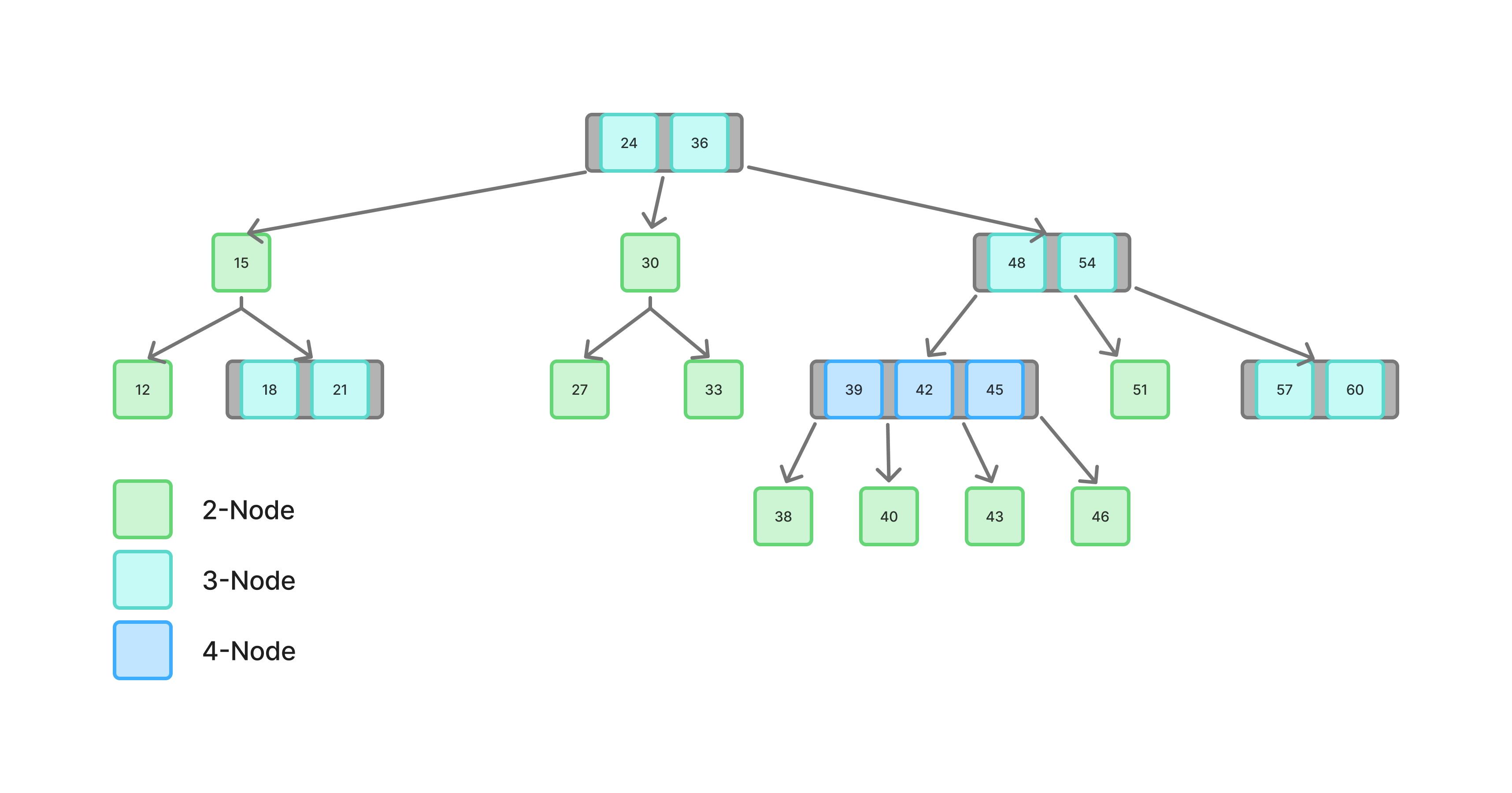

![:scale 90%](images/2-3-4-tree.png)

---

# Standard C++ containers

---

The C++ Standard Library defines two main *associative containers*, usually
implemented as Red-Black trees:

- `std::set`
    - Contains a sorted set of *unique* objects
    - Objects must be comparable, as they are used as keys directly
- `std::map`
    - Contains sorted pairs of key-value
    - Keys must be comparable and unique

???

- multiset, multimap can have multiple items with the same key
    - `find()` returns an iterator
- "unordered" version of set and map are implemented with hashtables

![:newline 2]
- Comparison with *sequence* containers (vector, list, etc.)
    - Logarithmic vs linear complexity
    - More complex to manage (balancing upon insertion/removal) and extra space
      per stored item (color, pointers to left/right children)
    - Collection remains always sorted, by design
    - Collection needs to be "big enough" to justify the extra complexity

---

## Set

.lcol66.small[

```C
#include <iostream>
#include <set>

int main() {
  // Initialization
  std::set<int> s = {7, 5, 16, 8};

// Add item dynamically
  s.insert(6);

// Add already existing item
  s.insert(8);

// Iterate and print values
  for (auto n : s)
    std::cout << n << std::endl;

return 0;
}

```

![:filename](std_set_example.cc)

]

.rcol33.small[
```terminal
5
6
7
8
16
```
]

---

## Map

.lcol66.footnotesize[

```C
#include <iostream>
#include <map>

int main() {
  // Initialization
  std::map<int, std::string> m = {
    {36, "Alice"}, {23, "Bob"}
  };

// Dynamic insertion by indexing
  m[8] = "Lisa";

// Dynamic pair insertion
  m.insert({10, "Bart"});

// Alternative pair insertion
  // and of duplicated item
  m.insert(std::make_pair(10, "Bart"));

// Iterate and print values
  for (auto n : m)
    std::cout << "(" << n.second
        << ": " << n.first << ")"
        << std::endl;

return 0;
}

```

![:filename](std_map_example.cc)

]

.rcol33.small[
```terminal
(Lisa: 8)
(Bart: 10)
(Bob: 23)
(Alice: 36)
```
]

---

# Comparison of self-balancing trees

From the general consensus:

### AVL trees
- Great if searching is the prevailing operation, because of stricter
  balance
- Insertion and removal can be somewhat slow

### Splay trees
- Great if large number of items but only a few are frequently accessed
- Poor with random accesses

### Red-black trees
- Best compromise
- Hence used in most libraries

### B-trees
- Great for on-disk data structures

![:newline 1]
#### Further info:
- <https://web.stanford.edu/~blp/papers/libavl.pdf>
- <https://www.google.com/search?q=avl+vs+red+black+vs+splay>